Documentation / Tutorials

Graph Visualisation

This tutorial is dedicated to visualisation of graphs and the addition and animation of data on graph renderings. As usual, it is cut in an informational part and a practical part at the end.

Stars

Viewer basics

Viewers

GraphStream does not provide one but several viewers.

From the 2.0 version of GraphStream, the default viewer is no part of the gs-core package anymore. Viewers are available separately. Viewers are located in gs-ui-TECH modules, where TECH is the name of the GUI tech used. To use it, you shall download the gs-ui-TECH.jar jar in the download section of the site and put it in your class path. These viewers support most of the GraphStream CSS reference:

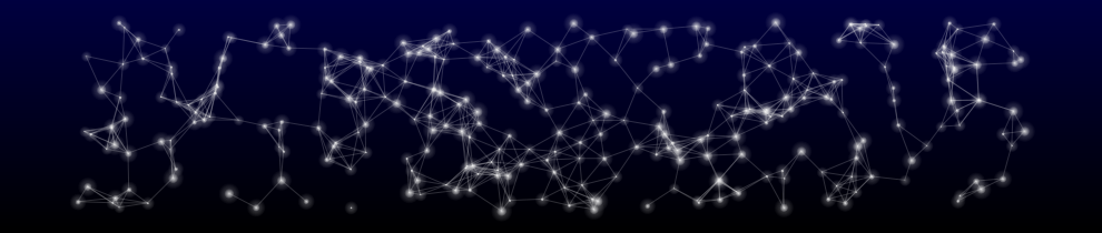
Several node and edge shapes,
Borders (fill and stroke),
Images,
Shadows,
Text positionning.

Fill mode scaled Shadow Radial Shadow Offset Icon Size Mode Node Shape Sprite Shape

How to display a graph

There are several ways to display a graph. The most easy one is to use the Graph.display() method. This is in fact a shortcut that creates a viewer for you. Indeed, its return value is an instance of the viewer used to display the graph. This method by default will try to place the nodes automatically in space to make the graph as readable as possible. You can also request that this automatic placement be disabled with Graph.display(boolean), passing the value false (however for your nodes to be visible, you therefore have to give them a position).

It is also possible to directly create the viewer by hand. This is often necessary in order to include the graph view inside your own GUIs, this is described under.

Please note that the display() method is not available on gs-ui-android, which requires to be embedded your own Android GUI.

You can specify which viewer to use by setting a global property named org.graphstream.ui. You can use the value swing or javafx depending on which GUI you want to use. This can be done in the main() method using the following code for example:

public static void main(String args[]) {
	System.setProperty("org.graphstream.ui", "swing");
	...
}

You can also pass this value directly to the JVM when launching the program:

java -Dorg.graphstream.ui=swing yourProgram

The value is a link of the display class to use, so swing is a shortcut for org.graphstream.ui.swing.util.Display. you can provide your own graph renderers if you wish. There is a org.graphstream.ui.swingViewer.GraphRenderer interface that you can follow to do this, but this is the matter of another tutorial.

The viewer

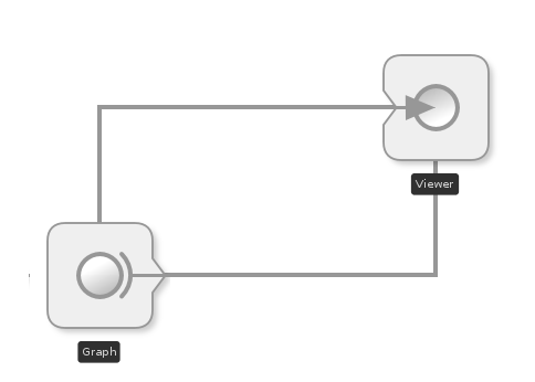
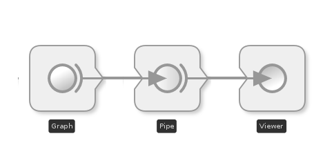
The Graph.display() method creates a new viewer and then connects it as a sink for graph events coming from the graph:

Diagram

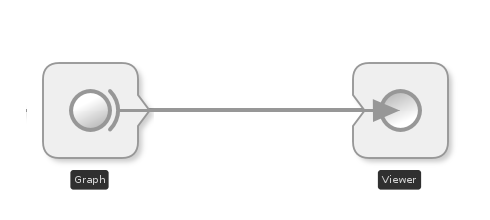
The viewer therefore receives each change occurring in the graph. In fact the viewer lives in another thread and the link between the graph and the viewer needs to accommodate this fact, this is discussed under.

The viewer created by the display() method is returned by this method:

Graph graph = new SingleGraph("I can see dead pixels");
Viewer viewer = graph.display();
....

Although the viewer runs in another thread, its public methods are protected from concurrent accesses, and you can safely call them from the default thread.

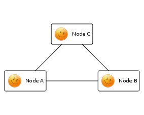
Automatic layout

As said above, the viewer will by default activate an automatic layout algorithm that will try to place the nodes so as to make the graph readable. The default automatic layout uses a force driven algorithm that makes all the nodes repel other nodes and a contradictory force that makes all nodes tied by an edge attract each other. The edges have a default length of one graph unit and try to fit this length. The result of this force algorithm is that the graph will tend to make nodes tied with each other close.

You can at any time activate or deactivate this layout, using the viewer:

Graph graph = new MultiGraph("Bazinga!");
// Populate the graph.
Viewer viewer = graph.display();
// Let the layout work ...
viewer.disableAutoLayout();
// Do some work ...
viewer.enableAutoLayout();

Coordinate system

There is no default coordinate system in GraphStream, you choose coordinates by yourself. If you choose to deactivate the automatic layout, the viewer will refuse to show your graph until you give nodes a position, indeed nodes will appear only once they have been positioned. You do this by setting one or more attributes on the node.

Most often the graph is represented in two dimensions, although a 3D viewer is in the works. You set the individual coordinates of a node using the x, y and z attributes, this way:

node.setAttribute("x", 1);
node.setAttribute("y", 3);

You can also use the xy or xyz attributes that take two or three values respectively:

node.setAttribute("xyz", 1, 3, 0);

You are encouraged to use the xyz attribute.

You fix the coordinates as you wish. The units you use will be called “Graph Units”. However, as you will see later, the viewer supports two other units: pixels and percents. They are most often used to describe styling rules, but can also be used to position sprites.

Sprites

Sprites are informational symbols that you can add to the graph display. Internally, they are merely attributes stored on nodes, edges or the graph itself. However these attributes have a specific form understood by the viewers that allow to describe their type and their position.

A sprite can be freely positioned on the viewer canvas as a node would be. They allow to place symbols, labels, icons, shapes in the graph rendering. However an interesting property of sprites consist in “attaching” them to a node or edge. When attached, their position is expressed relative to the graph element they are attached to.

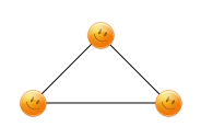
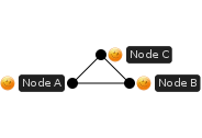
For example a sprite attached to a node uses “spherical” coordinates to describe its position. Its first coordinate is a radius (a distance from the node center), its second coordinate and angle of rotation around the node center in the XY plane, and its optional third coordinate describe an angle around the node center in the XZ plane (the Z axis going “out” of the screen, perpendicular to it).

Spherical Coordinate System

Here is an example of a sprite attached to a node A with first coordinate 10px (radius) and second coordinate 30 (degrees).

Node Coordinates

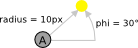
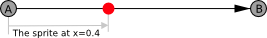
When attached to an edge, a sprite position is a real number between 0 and 1 that describe its “advance” on the edge. At position 0 the sprite is on the source node, at position 1 it is on the target node, and for example at position 0.5 it is in the middle of the edge.

Edge Coordinates

Sprites can have the same shapes as nodes, but also provide several other useful shapes.

Sperite Shape

Although sprites are stored as attributes, this is not a very convenient way to deal with them. In order to ease sprite management, a org.graphstream.ui.spriteManager.SpriteManager class is provided. When you create such an object, it will start to observe the graph and allow you to add, change and remove sprites on it. It is able to retrieve the sprites already stored as attributes on the graph, for example if you read the graph from a file:

import org.graphstream.ui.spriteManager.*;
// ...
Graph graph = new MultiGraph("Live long and prosper");
// ...
SpriteManager sman = new SpriteManager(graph);

Then you can easily add sprites on the graph:

Sprite s = sman.addSprite("S1");

Sprites are identified by a unique string, like nodes and edges. The addSprite() method returns a dummy object that allows to handle the sprite. This object is an interface that will modify the attributes stored on the graph for you.

You can position the sprite using for example:

s.setPosition(2, 1, 0);

This will place the sprite at an absolute Cartesian position (2,1,0). To attach a sprite to a node you can use:

s.attachToNode("A");

This will inform the renderer that the sprite position is relative to the node A position. In this case, as said above, the position is expressed in spherical coordinates. This allows the sprite to “orbit” around the node. Therefore its three coordinates indicate first a radius (a distance between the sprite and the node center), then two angles of rotation around the node center, one in the XY plane, the other in the XZ plane.

The method:

s.attachToEdge("AB");

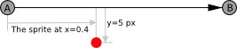
Allows to attach a sprite to an edge. When attached, once again, the coordinates are expressed “along” the edge. The first value express the advance of the sprite on the edge. Its values must be taken between 0 and 1 included. Using it, by slowly increasing the value, you can make the sprite move along the edge for example. The second coordinate express a distance between the sprite and the edge, perpendicular to it.

Edge coordinates

The third coordinate express a rotation angle around the edge, the edge being the rotation axis. For sprites attached to edges, it is often useful to specify only the first coordinate:

s.setPosition(0.5);

This will put the sprite just in the middle of the edge AB.

To detach the sprite and position it anew in absolute Cartesian coordinates, use:

s.detach();

The length units used to position sprites are graph units, as for nodes. This includes the absolute position of sprites that are not attached to a graph element, the distance of a sprite attached to a node, or the distance of a sprite attached to an edge. However, it is sometimes useful to specify length coordinates using pixels or percents. You can do this using:

import org.graphstream.ui.graphicGraph.stylesheet.Style.Units;
// ...
s.attachToNode("A");
s.setPosition(Units.PX, 12, 180, 0);

As you can see, you can change the attachment of a sprite at any time, it is therefore easy to simulate the displacement of elements in the graph.

Sprites are treated as any other graph element, and therefore, like nodes and edges can have an arbitrary number of attributes. You set and change the attributes using the same methods as for nodes and edges, indeed, the Sprite class inherit Element.

The GraphStream CSS

The graph describes the structure to be rendered by the viewer. It is often not very interesting to store directly in the graph styling rules that change the appearance of the display. Usually, attributes are used to store data according to an algorithm you are working on for example, but you do not want to burden yourself with stylistic details at this point.

Therefore, to change the appearance of elements in the viewer, GraphStream defines a kind of style sheet using the same syntax as the cascading style sheets (CSS) of HTML. In this way the structure of the graph is completely separated from its appearance.

There are some attributes that control the display however, since it is not always possible to avoid them. Most of these attributes starts with the prefix ui.. The first of these attributes you need to know is the one that specify the style sheet to use: ui.stylesheet. This attribute must be stored on a graph and takes as value either the style sheet itself as a string of characters or the URL of a file, local, distant or packaged in a jar.

You can for example change the background color of the graph using a style sheet given as a string this way:

graph.setAttribute("ui.stylesheet", "graph { fill-color: red; }");

But you can also specify an URL:

graph.setAttribute("ui.stylehseet", "url('http://www.deep.in/the/site/mystylesheet')");

Or:

graph.setAttribute("ui.stylesheet", "url(file:///somewhere/over/the/rainbow/stylesheet')");

The style sheets are cumulative, each time you change the ui.stylesheet attribute, the new style sheet is read and merged with the previous ones, replacing or adding style definitions. You can however completely clear the style of a graph using:

graph.removeAttribute("ui.stylesheet");

The syntax of a style sheet is very similar to the one seen in the cascading style sheets of HTML. The CSS of GraphStream mostly follows the same rules, including inheritance and composition of styles. A style sheet is a sequence of styling rules. A styling rule is made of a selector and a set of style properties.

There are four main selectors graph, node, edge and sprite. They allow to define rules that applies to a global set of elements. However you can specialize these selectors by identifying a specific element, for example the node with identifier A can be selected using node#A. You can also define classes of elements. For example, all nodes with class zo can be matched by node.zo. You can assign a class to a node using the attribute ui.class whose value must be a string containing a coma separated list of class names. Therefore nodes can pertain to several classes, the style of the classes being aggregated.

Following the selector, you give a set of styling properties between curly braces. The styling properties are made of a property name followed by a colon : then one or more values separated by comas, and finished by a semi-colon ;.

Here is an example of a complete styling rule for a node whose identifier is A whose shape is a box, side size is 15 pixels on 20 pixels, fill color is red and border color blue (who said styling is related to style ?):

node#A {
	shape: box;
	size: 15px, 20px;
	fill-mode: plain;   /* Default.          */
	fill-color: red;    /* Default is black. */
	stroke-mode: plain; /* Default is none.  */
	stroke-color: blue; /* Default is black. */
}

First stylesheet

Note that the semi-colon is mandatory, even if there is only one property.

There are a lot of style properties, some applies only to a kind of selector. They are described in the CSS reference, which describes the whole set of style properties available in GraphStream. Do not forget that not all the CSS properties are supported in all the viewers. These gs-ui-Z viewers understands most of the properties listed in the CSS reference.

Rendering quality

The swing viewer supports several rendering modes. Both the simple and advanced viewers have two options to tune quality. The first one is set by adding the ui.quality attribute to the graph. This attribute does not need a value. It informs the viewer that it can use rendering algorithms that are more time consuming to favor quality instead of speed:

graph.setAttribute("ui.quality");

The other attribute allows to activate anti-aliasing of lines and shapes, simply put it on the graph:

graph.setAttribute("ui.antialias");

Removing these attributes will restore the default behavior.

Rendering speed

Most of the time, the Java2D viewers drawing performance can degrade quickly when the number of nodes and edges grows. This is due to the all-CPU pure Java graphics renderer used by default on some platforms. You can greatly improve their performance by activating graphic acceleration. This can be done for example using the following options:

java -Dsun.java2d.directx=True on Windows. On newer versions of windows this should be activated by default.
On OS X hosts, by default the quartz renderer is activated.
java -Dsun.java2d.opengl=True on Linux. Sadly it is not activated by default.

In android, you can enable or disable the hardware acceleration in the Manifest.

<application
	...	
	tools:replace="android:hardwareAccelerated">

But be careful, some CSS property effect may changes.

Advanced view

This section can be skipped at first if you are only interested in representing the graph. It deals with the integration of the viewer in your own GUIs, of the retrieving of mouse clicks on nodes, and on the way to control the viewer views. It requires a good understanding of Swing and the way it handles events, in its own thread.

Integrating the viewer in your GUI

In order to integrate the viewer in a Swing GUI, you will need to create the viewer by yourself. The viewer handles a set of views of the graph (this has been done to allow a view for the graph itself, but also views for data or statistics. Actually, only the graph view is available however). Once the viewer is created you can add a view and request that it is not automatically inserted in a window frame (a JFrame). All views, instance of View, inherit from JPanel and therefore can be embedded in Swing GUIs.

Here is how you do that:

import org.graphstream.ui.swingViewer.View;
import org.graphstream.ui.swingViewer.Viewer;
// ....
Graph graph = new MultiGraph("embedded");
Viewer viewer = new Viewer(graph, Viewer.ThreadingModel.GRAPH_IN_ANOTHER_THREAD);
// ...
View view = viewer.addDefaultView(false);   // false indicates "no JFrame".
// ...
myJFrame.add(view);

The Viewer.ThreadingModel.GRAPH_IN_ANOTHER_THREAD constant informs the viewer that you will continue to use the Java main thread, while the GUI runs in its own thread (The Swing of AWT thread). Be very careful with this, since this means some synchronization will occur between the two threads. We will come back on this topic later.

Controlling the view, the `View` API

Even if you did not created the view yourself, you can always access the default view created for you, for example:

Viewer viewer = graph.display();
View view = viewer.getDefaultView();

The View interface defines a ‘camera’ object that has several methods allowing you to navigate the graph rendering (the camera object is synchronize and allows to command the view even from a distinct thread). By default the view is in a mode where it adapts to the graph size to always show the entire graph and so that the center of the view is at the center of the graph. However you can leave this mode at any time to specify the point at the center of the view (in order to “move in the graph”) using for example:

view.getCamera().setViewCenter(2, 3, 4);

You can also zoom in or out using:

view.getCamera().setViewPercent(0.5);

This will zoom of 200% on the view center.

However in this mode, if the graph changes, if the nodes move, the view will remain centered on the point you given, with the zoom you given. To restore the automatic fitting of the zoom and center for the graph, use:

view.getCamera().resetView();

Drawing in the graph viewer

You can also add a back and fore layers in the graph view where you can draw using the Graphics2D API. This is done using View.setBackLayerRenderer() and View.setFrontLayerRenderer(). You give to these methods an object that implement the LayerRenderer interface. This interface is composed of only one method:

void render(Graphics2D graphics, GraphicGraph graph, double px2Gu,
    int widthPx, int heightPx, double minXGu, double minYGu,
    double maxXGu, double maxYGu);

This method takes a Graphics2D, a special graph instance of GraphicGraph, containing the graph that is actually drawn, with additional graphic information like node position, an GraphicSprite objects representing the sprites to draw, as well as a StyleSheet object. The method also takes a scaling factor px2Gu that allows to pass from pixels to graph units and inversely. Then the width and height of the view in pixel are given (the graph may not fill the entire view due to its aspect ratio being different from the one of the panel). Finally, you receive the bounds of the graph in graph units.

The back layer is rendered before the graph is drawn, and the fore layer is drawn after the graph is rendered. Using this mechanism, you can draw anything on or under the graph according to the information in the graphic graph. The GraphicGraph implements Graph but is not a fully blown graph and some operations are not possible on it, however you can iterate on its elements, which are of type GraphicNode, GraphicEdge and GraphicSprite.

Retrieving mouse clicks on the viewer

Here we have several ways to work. It depends on the program you intend to create:

If you plan to do a GUI only program, that is a program that only respond to GUI events (mous clicks, keyboard, etc.) you should work in the GUI thread, using listeners.
If you intend to create some sort of simulation that runs a code continuously on the graph and uses the viewer to display its results, you should work in the Java main thread (created when you launch the program) and comunicate with the viewer GUI.

Please note that by default, some features have been disabled in order to save resources These include the edge selection, the mouseOver, and mouseLeft functions. If you want to activate them, you can use the enableMouseOptions method of View:

viewer.getDefaultView().enableMouseOptions();

This is a shortcut used to replace the default mouse manager. You can also do it manually :

viewer.getDefaultView().setMouseManager(new MouseOverMouseManager(EnumSet.of(InteractiveElement.EDGE, InteractiveElement.NODE, InteractiveElement.SPRITE)));

Working in the GUI thread

The first case is the most simple, you work like in most Swing or AWT programs: in an event based manner, waiting for listeners to be called by the GUI.

In this case you have to create the viewer using another threading model :

Viewer viewer = new Viewer(graph, Viewer.ThreadingModel.GRAPH_IN_SWING_THREAD)

We will explain in the next section how to work in parallel with the GUI and allow syncronization between a graph in the Java main thread and the GUI, but here we disable this mechanism, telling the viewer that the graph and the GUI will be handled in the same thread. This is a little faster.

Simulations and GUI views

Doing all in Swing is not necessarily a good idea however, this works for small programs, but for others, you will want the graph to be handled by a special thread that do its work in parallel of the GUI to not freeze it. If you have several processor cores, or several processors (even phones have now), this is good.

Retrieving events occuring on the viewer requires us to connect the graph as a sink for the viewer. Indeed, events are propagated as attributes in the graph. These attributes will, as usual begin with the prefix “ui.”.

Making the graph as a sink of the viewer, creates a loop. As we already have seen it, the viewer is a sink for the graph. What will happen thus, is a kind of synchronisation of the two elements, the graph and the viewer graph representation. When one change, the change will be propagated to the other.

Diagram

However, the graph and the viewer do not run in the same thread. Until now this has been completely transparent. However to retrieve the graph events coming from the viewer, we will have to explicitly request them to be sent regularly. Furthermore, we will not be able to put our graph directly as sink of the viewer, we will need to create a special pipe that allows inter-thread communication.

When you only want to display a graph, a similar mechanism is used but transparently: the viewer is not directly sink of the graph, a special pipe is created between the two. This pipe role is to cross the inter-thread barrier properly. All this mechanism is hidden and done for you. It is important and interesting since it allows you to work on the graph in the default thread of Java while the viewer displays your work in the Swing thread in parallel. Most computers having several cores nowadays, this allows to better use them (naturally, you can override this behavior, as it will be demonstrated later).

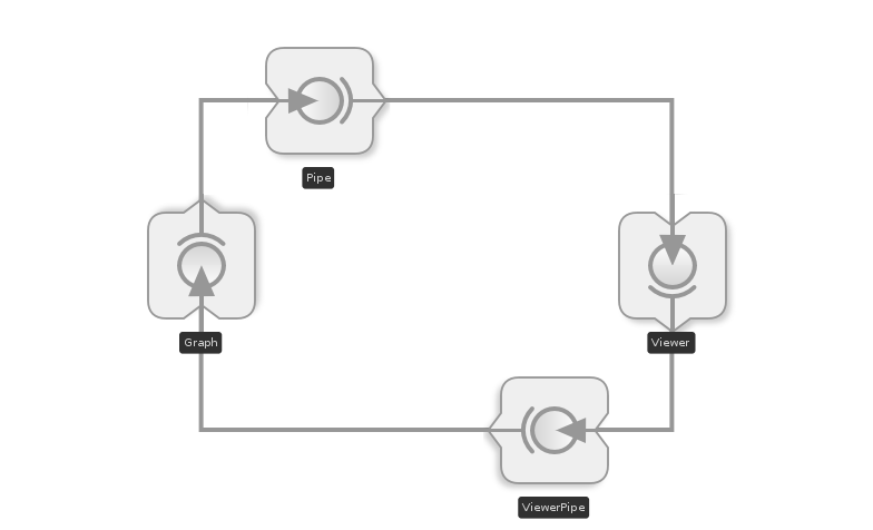
Here is the real situation we have when we display a graph, a special pipe is used to cross the thread boundaries:

Diagram 2

Now to close the loop we need some kind of pipe to retrieve the events from the viewer. This is the role of the Viewer.newViewerPipe() method. It will return the pipe object of type ViewerPipe that will act as source for events coming from the viewer. You need to connect your graph to it:

Diagram 3

However you will also need to regularly ask this pipe to look if the viewer thread sent some events, this cannot be done automatically easily, so you have the responsibility to do it. This is done by calling the ViewerPipe.pump() method. A ViewerPipe.blockingPump() method is also available in the nightly builds.

The events coming from the viewer are simple attributes. You could observe your graph for changes occurring on it, looking for these events, but this is not very easy. Therefore, the ViewerPipe can register listeners of type ViewerListener, and send them events by calling their methods when some event attributes are changed.

Let’s see an example:

public class Clicks implements ViewerListener {
	protected boolean loop = true;

	public static void main(String args[]) {
		System.setProperty("org.graphstream.ui", "swing");
		new Clicks();
	}
	public Clicks() {
		// We do as usual to display a graph. This
		// connect the graph outputs to the viewer.
		// The viewer is a sink of the graph.
		Graph graph = new SingleGraph("Clicks");
		Viewer viewer = graph.display();

		// The default action when closing the view is to quit
		// the program.
		viewer.setCloseFramePolicy(Viewer.CloseFramePolicy.HIDE_ONLY);

		// We connect back the viewer to the graph,
		// the graph becomes a sink for the viewer.
		// We also install us as a viewer listener to
		// intercept the graphic events.
		ViewerPipe fromViewer = viewer.newViewerPipe();
		fromViewer.addViewerListener(this);
		fromViewer.addSink(graph);

		// Then we need a loop to do our work and to wait for events.
		// In this loop we will need to call the
		// pump() method before each use of the graph to copy back events
		// that have already occurred in the viewer thread inside
		// our thread.

		while(loop) {
			fromViewer.pump(); // or fromViewer.blockingPump(); in the nightly builds

			// here your simulation code.

			// You do not necessarily need to use a loop, this is only an example.
			// as long as you call pump() before using the graph. pump() is non
			// blocking.  If you only use the loop to look at event, use blockingPump()
			// to avoid 100% CPU usage. The blockingPump() method is only available from
			// the nightly builds.
		}
	}

	public void viewClosed(String id) {
		loop = false;
	}

	public void buttonPushed(String id) {
		System.out.println("Button pushed on node "+id);
	}

	public void buttonReleased(String id) {
		System.out.println("Button released on node "+id);
	}

	public void mouseOver(String id) {
		System.out.println("Need the Mouse Options to be activated");
	}

	public void mouseLeft(String id) {
		System.out.println("Need the Mouse Options to be activated");
	}
}

Retrieving nodes coordinates of the automatic layout

The automatic layout process, when activated, only send nodes position to the viewer (however Layout is an algorithm, and you could create it by yourself and apply it to your graph if you want). Therefore your graph will not be modified by this layout process, and the computed node positions will not be stored in the graph. This is a wanted behavior, the viewer, by default, will not interfere with your graph.

As explained in the previous section, making the graph a sink of the viewer will allow this graph to be synchronized with the viewer graph representation. Each change to the graph will be copied to the viewer and inversely. Therefore the computed node positions will also be copied. And thus you have no more action to do than to call ViewerPipe.pump() to retrieve these values.

The org.graphstream.algorithm.Toolkit class contains utility methods to easily retrieve node positions. You can do for example something like this:

import static Toolkit.*;
...
Node node = graph.getNode("SomeId");
double pos[] = nodePosition(node);
...

An example: drawing GIS Data

Geographical Information Systems among other things allow to manipulate geographic data and render it. Most often the data is stored under a form that is difficult to use for simulations. What one could want for example is to extract the road network of GIS data under the form of a graph. GraphStream provides a module to do that. We propose you to use the data collected by this module to render a map of a city with the GraphStream viewer. In a first step we will see how to add some style to the city map. In a second time, we will add a very basic traffic simulation on the map and the underlying road graph.

But before that, we will need to add the viewer we use. We are going to use gs-ui-swing for this example. To add this viewer, we can write the following line right at the beginning of the program, before the graph creation:

System.setProperty("org.graphstream.ui", "swing");

You must ensure you have the gs-ui-swing.jar jar in your classpath to use this new viewer.

The data

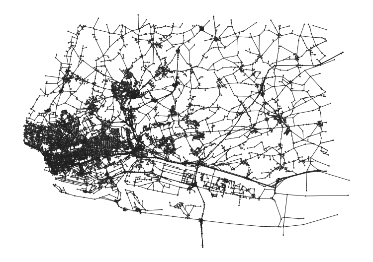
You will find at the following URL a graph in the DGS format that describes the road network of the city of Le Havre in France:

Graph of the road network for the city of Le Havre

Save it under the name “LeHavre.dgs”. This graph can be loaded and displayed easily:

public class LeHavre {
	public static void main(String args[]) {
		System.setProperty("org.graphstream.ui", "swing");
		new LeHavre();
	}
	
	public LeHavre() {
		Graph graph = new MultiGraph("Le Havre");
		
		try {
			graph.read("LeHavre.dgs");
		} catch(Exception e) {
			e.printStackTrace();
			System.exit(1);
		}
		
		graph.display(false);   // No auto-layout.
	}
}

This creates a multi-graph (a graph where several edges can exist between two same nodes), and tries to read it. When reading a graph, you must be prepared to an eventual I/O error or parsing error, this is why the Graph.read() method is surrounded by the annoying try-catch block.

If successful, we display the graph using the Graph.display() method, passing it a Boolean argument specifying that we do not want the viewer to try to layout the graph by automatically positioning the nodes. Indeed in the given graph, all nodes have a geographic location specified using the xyz attribute.

However, as you will notice, the display is not quite appropriate when displaying a map. First nodes are rendered as large black dots that cover most of the edges. Furthermore, the data provides a label for each node and an annoying text is added on each intersection.

Le Havre Step 1

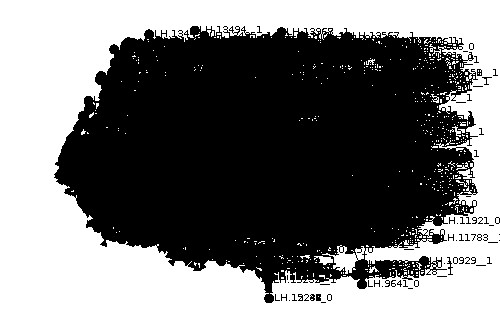
So let’s add some style to correct this !

A first style sheet

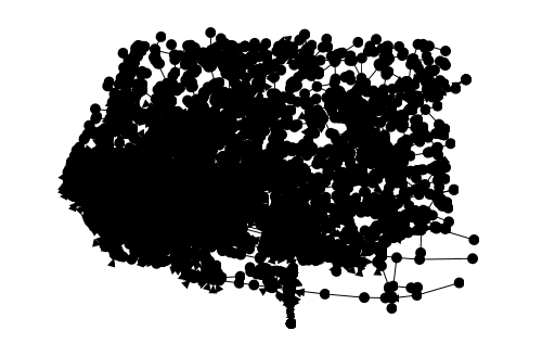
We will first make the display a cleaner hiding text by default. Here is the style sheet we will use:

node {
	text-mode: hidden;
}

We can modify the program to use this style sheet by adding it as an attribute ui.stylesheet:

public class LeHavre {
	public static void main(String args[]) {
		System.setProperty("org.graphstream.ui", "swing");
		new LeHavre();
	}
	
	public LeHavre() {
		Graph graph = new MultiGraph("Le Havre");
		
		try {
			graph.read("LeHavre.dgs");
		} catch(Exception e) {
			e.printStackTrace();
			System.exit(1);
		}
		
		graph.setAttribute("ui.stylesheet", styleSheet);
		graph.display(false);   // No auto-layout.
	}
}

Le Havre Step 2

However, this is still not really readable. Let’s change the node size, and add some colors. This is not really visible, but as some streets are one way only, there are arrows on some edges, they also are too large, so we will give them a new size.

Furthermore, we are interested mainly in the road network, and therefore in the edges of the graph, the nodes represent intersection points. By default the viewer draws first the edges, then above the edges the nodes (and eventually above the nodes, it draws the sprites). However, it could be useful here to make the nodes appear under the edges. This is possible using the z-index style property. By default this property is set to 1 for the edges and 2 for the nodes (a higher z-index means that it is drawn above the others). In the style sheet we therefore set the z-index of the nodes to 0 in order to draw the nodes under the edges.

Modify the style sheet to look like this:

node {
	size: 3px;
	fill-color: #777;
	text-mode: hidden;
	z-index: 0;
}

edge {
	shape: line;
	fill-color: #222;
	arrow-size: 3px, 2px;
}

In addition, we will position two other attributes on the graph ui.quality and ui.antialias that will help beautifying the display in gs-ui-swing. Above the line that adds the ui.stylesheet attribute add the two lines:

graph.setAttribute("ui.quality");
graph.setAttribute("ui.antialias");

Le Havre Step 3

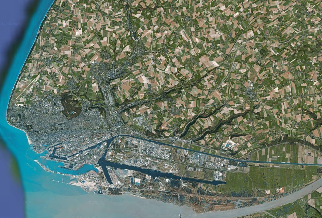
To help you see how the above graph relates to the city, here is a screen shot of the same area done using Google Maps:

Le Havre Step 0

Adding style classes

We will now change the appearance of some edges according to some attributes stored on these edges. There are a lot of data in the graph you downloaded. For each edge, there are three attributes that specify if an edge is a bridge with isBridge, a tunnel with isTunnel or a tollway with isTollway. These attributes are present only if the corresponding edge is indeed a bridge, a tunnel or a tollway. Therefore we will browse all edges of the graph to look at these attributes in order to change the way they look.

Until then, we only changed the style of the whole set of edges or the whole set of nodes. To change only some elements, we can use style classes. A class is a style that is applied to an element only if it has an attribute ui.class which contains the name of the style class. For example in order to make an edge pertain to the tollway class, one can use:

edge.setAttribute("ui.class", "tollway");

An element may pertain to several style classes in which case the styles are merged, with a priority to classes that appear first in the list. The list is separated by comas. For example if an edge pertains to two classes you can write:

edge.setAttribute("ui.class", "tollway, foo");

In the style sheet, you specify the style for a class using for example:

edge.tollway { size: 2px; }

Such a style is applied in cascade with the style for each edge. This means that an edge with the tollway class for example will have the style of each edge, plus the style defined by the edge.tollway style. If the two styles define the same properties, the class style is chosen.

First, we will add the classes attributes on the edges, just after the graph reading try-catch block, add the following code:

graph.edges().forEach(edge -> {
	if(edge.hasAttribute("isTollway")) {
		edge.setAttribute("ui.class", "tollway");
	} else if(edge.hasAttribute("isTunnel")) {
		edge.setAttribute("ui.class", "tunnel");
	} else if(edge.hasAttribute("isBridge")) {
		edge.setAttribute("ui.class", "bridge");
	}
});

This code will iterate on each edge of the graph. If an edge has one of the attributes listed above, we add it one of the three classes tollway, tunnel or bridge.

Then we will add in the style sheet the three style classes:

edge.tollway { size: 2px; stroke-color: red; stroke-width: 1px; stroke-mode: plain; }
edge.tunnel { stroke-color: blue; stroke-width: 1px; stroke-mode: plain; }
edge.bridge { stroke-color: yellow; stroke-width: 1px; stroke-mode: plain; }

Each of these classes add a border around the edges with a distinct color, red for tollways, blue for tunnels, and yellow for bridges.

Le Havre Step 4

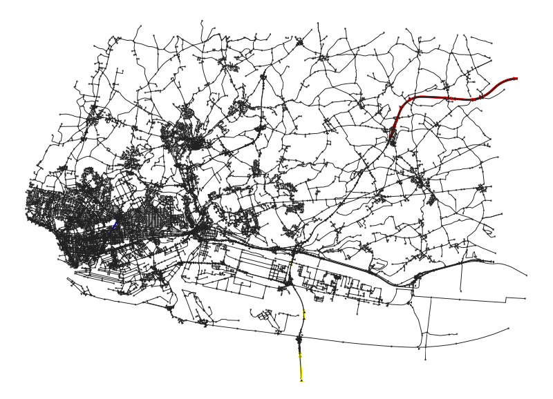
There are few bridges in the city, on the south east, you can see three bridges that cross the Le Havre canal, the harbor, and finally the Normandy Bridge above the Seine river. There is only one tunnel, in blue, and finally one tollway on the north east.

Zooming and panning

You may not well see the tunnel in blue. At the scale of the city, it is finally small (300 meters). However you can instruct the viewer to zoom on the view and to move to a given point of view. This is done by accessing the Viewer object and the actual View it is using. Indeed, the viewer may have several views on the same graph.

The Graph.display() method returns a reference on the viewer used for display. The returned object if of type Viewer. This viewer provides lots of methods allowing to control the viewer and its views. To obtain the default view used to display the graph, you can use the Viewer.getDefaultView() method. The View object in turn allows to control the frame size (it can be embedded in a GUI without this frame if needed), the zoom and the looked at point inside the graph via the camera. This is done using the View.resizeFrame(), Camera.setViewPercent() and Camera.setViewCenter() methods.

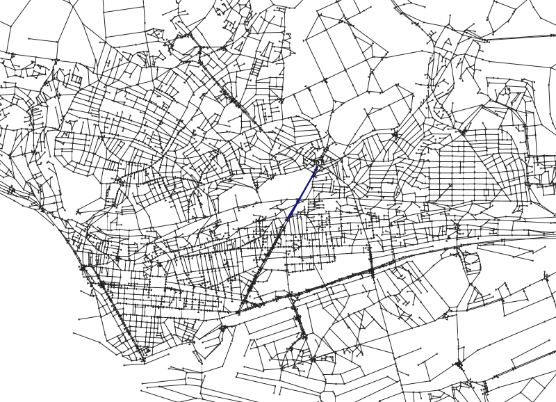
Replace the graph.display(false); statement in your code by the following lines:

Viewer viewer = graph.display(false);
ViewPanel view = (ViewPanel) viewer.getDefaultView(); // ViewPanel is the view for gs-ui-swing
view.resizeFrame(800, 600);
view.getCamera().setViewCenter(3000, 8000, 0);
view.getCamera().setViewPercent(0.25);

The setViewCenter method takes three arguments since views can be 2D but also 3D. Here we work in two dimensions only, hence the last argument set to zero. The setViewPercent method takes as argument a double that tells which percent of the whole graph is visible. For example, the value 0.5 shows only half of the graph.

Now, we are able to better see the tunnel, with edges in black representing the roads that pass above it.

Le Havre Step 5

When using the viewer interactively, you can also zoom and pan the view using the page-up and page-down keys to zoom and the arrow keys to pan. Notice that, when the graph is dynamic and change with tilen usually the view follows the graph size. In other words, the view automatically change the view center and the zoom to always show the whole graph. As soon as you start to change the zoom or move the view, the view will switch to a mode where it do not automatically update these settings. To switch back to automatic settings, you can use shift-R interactively or call View.resetView(). This is especially true if you want to change the element color or size inside a range of values according to some changing computation.

Imagine for example we want to color the edges according to a real-time traffic information. Let’s say for example we want to tint edges in green when the traffic is low, in yellow when the traffic grows, and in red when the traffic is high. We could use three style classes, but it would be interesting to have a gradient from green to yellow and from yellow to red to better show the traffic importance, according to the real numbers.

Dynamically changing colors and size

Using classes to change the appearance of some elements is useful. However if you need to often change the appearance of an element based on some computation you are doing on the graph it could become tedious.

Imagine for example you want to change the color of edges according to the traffic on the corresponding road. You want to tint the edge in red if the traffic is high, and make it more yellow if normal, coloring it in green when there is no traffic at all. To make things more readable, you want to use a gradient from red to yellow, and from yellow to green to indicate various degrees of congestion on the road.

It would not be a good solution to define a style class per color of the gradient from red to green. Instead we could use a special coloring mode of the GraphStream CSS named dynamic coloring. When using dynamic coloring, you define not one but several colors for the fill-color style property and set the fill-mode style property to the value dyn-plain. This indicates to the viewer that the color of the element will be one of the colors defined by fill-color or a gradient between these colors, depending on an attribute ui.color defined on the element. The value of this attribute must be a double between 0 and 1.

For example if you define two colors for fill-color, say red and yellow, and if the value of ui.color is 0 the element will be red. If the value is 1 the element will be yellow. And finally, if the value is 0.5 the element will be orange. Similarly, if you define three colors for fill-color the values for ui.color are still between 0 and 1, and the final color will be an interpolation of the colors, with special values 0 for the first color, 0.5 for the second color and 1 for the last color. You can use as many colors as you want.

The interesting part with this coloring method, is that you can change dynamically the values for the ui.color attribute on the graph elements.

The data stored on the graph you have does not incorporate traffic, but it contains maximum speed limits stored as a speedMax attribute on edges. We could use dynamic coloring to assign a specific color for each edge depending on its speed limit. The maximum speed limit in France is 130 kilometers per hour. Let’s first add the ui.color attributes on each edge. Inside the loop on each edge where we assign the tollway, bridge and tunnel classes, add:

graph.edges().forEach(edge -> {
	if(edge.hasAttribute("isTollway")) {
		edge.setAttribute("ui.class", "tollway");
	} else if(edge.hasAttribute("isTunnel")) {
		edge.setAttribute("ui.class", "tunnel");
	} else if(edge.hasAttribute("isBridge")) {
		edge.setAttribute("ui.class", "bridge");
	}

	// Add this :
	double speedMax = edge.getNumber("speedMax") / 130.0;
	edge.setAttribute("ui.color", speedMax);
});

This obtains the value stored in the speedMax attribute, expecting it is a number (which should be the case!) and divides this number by 130 to scale the value in the range 0 to 1. Then this value is used to put the ui.color attribute on the edge.

Next we will need to change the style sheet. Locate the edge definition, and replace the fill-color: #222; by the two fill-mode and fill-color lines, as shown under:

edge {
	shape: line;
	fill-mode: dyn-plain;
	fill-color: #222, #555, green, yellow;
	arrow-size: 3px, 2px;
}

This uses a gradient from almost black for very slow areas, to grey for urban areas, green for small roads and yellow for highways. Also, to make things more readable, we will also change the size of nodes:

node {
	size: 1px;
	fill-color: #777;
	text-mode: hidden;
	z-index: 0;
}

Remove or comment the lines that zoom and pan the view. You should obtain something like this:

Le Havre Step 6

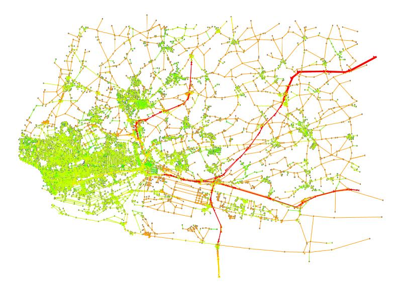
Urban areas appear in gray as speed limit is (hopefully) for more limited in these zones.

For an example that can easily be transformed to a dynamic update of the edge colors, see Random Walks on Graphs.

The dynamic change on colors is also available for the size of elements. Simply set the size property to the value dyn-size, then store a ui.size attribute on elements. The size is in graph units.

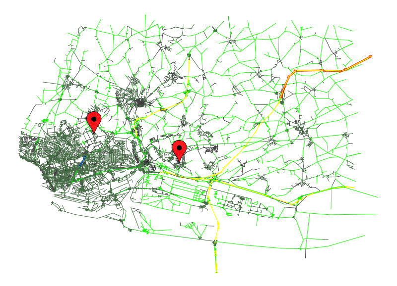
Adding some symbols

Sometimes, it is useful to add some symbols on a graph rendering in addition to the nodes and edges.

For example, in our map of the Le Havre city, one could want to display pins to indicate a particular position. This can be done using sprites.

A sprite is like a node and an be positioned everywhere in the viewer space. Unlike nodes however, sprites have the ability to attach to nodes or edges in order to express their position according to the element they are attached to. Sprites are in fact stored as attributes on the graph, they do not really exist as objects. This allows to save the sprites in the graph event flow for example.

To manage sprites you can use the SpriteManager class. This class takes a graph as argument of its constructor. If there are already some sprite attributes on the graph, the sprite manager will retrieve them. The sprite manager also allows to create new sprites, and in returns provide a Sprite class that allows to easily set sprites properties, like the position for example or the attachment.

Just after the loop that process each edge in our program, add the following code:

SpriteManager sman = new SpriteManager(graph);
Sprite s1 = sman.addSprite("S1");
Sprite s2 = sman.addSprite("S2");

This will create the sprite manager and add two sprites S1 and S2.

Then we will try to position the sprites on two nodes of the graph We can do this by randomly choosing two nodes, obtaining their current position to assign it to the sprites. The Toolkit class of the gs-algo package provides a way to randomly pick a node in a graph. Most methods of Toolkit are utility methods declared as static methods. Therefore to use them, the better way is to use a static import (available in Java 1.6):

import static org.graphstream.algorithm.Toolkit.*;

Then just after the two sprites creation code, add:

Node n1 = randomNode(graph);
Node n2 = randomNode(graph);
double p1[] = nodePosition(n1);
double p2[] = nodePosition(n2);
s1.setPosition(p1[0], p1[1], p1[2]);
s2.setPosition(p2[0], p2[1], p2[2]);

The nodePosition() method is an utility method also defined in Toolkit that returns an array of three doubles containing the value for the xyz attribute of a node. The Sprite.setPosition() method is then used with the retrieved node coordinates to position the sprite on the node.

The sprites will appear, by default, as black circles, like nodes without CSS style. We will therefore extend our style sheet to add:

sprite {
	shape: box;
	size: 32px, 52px;
	fill-mode: image-scaled;
	fill-image: url('mapPinSmall.png');
}

This apply to all sprites the shape box with the size of the image we want to draw:

Map Pin

Save this image to the directory of your program, or modify the URL in the style sheet, then run the program:

Le Havre Step 7

Taking a screen shot

Once your proud of your visualization, you can take a screen shot of the viewer at any time. You have several options for doing this, one is to use the FileSinkImage (described here), but another very simple way of doing this is to put a special attribute on the graph: ui.screenshot. The value of this attribute must be the file name of the screen shot image you want to save. The known extensions are jpg, png and bmp. The viewer will intercept this attribute, output the screen shot and remove the attribute.

For example:

graph.setAttribute("ui.screenshot", "/some/place/screenshot.png");

What about Android ?

Android is a bit peculiar since it doesn’t have a default display method. You need to create your own view in order to use it. For the convenience of the users, a default Android Fragment is provided. The Fragment can be used like so:

public void display(Bundle savedInstanceState, Graph graph, boolean autoLayout) {
    if (savedInstanceState == null) {
        FragmentManager fm = getSupportFragmentManager();

        // find fragment or create it
        fragment = (DefaultFragment) fm.findFragmentByTag("fragment_tag");
        if (null == fragment) {
            fragment = new DefaultFragment();
            fragment.init(graph, autoLayout);
        }

        // Add the fragment in the layout and commit
        FragmentTransaction ft = fm.beginTransaction() ;
        ft.add(CONTENT_VIEW_ID, fragment).commit();
    }
}

Of course, you can create your own UI with your own fragment. In that case, you have to follow a certain order in the construction of the graph view corresponding to the lifecycle of your Activity/Fragment. Three steps are necessary:

Create the viewer
Link the context
Create the view

Here the default Fragment, following the different steps :

...
	/**
	* 1- Create only one Viewer
	* @param savedInstanceState
	*/
	public void onCreate(@Nullable Bundle savedInstanceState) {
		super.onCreate(savedInstanceState);
		viewer = new AndroidViewer(graph, AndroidViewer.ThreadingModel.GRAPH_IN_ANOTHER_THREAD);
	}

	/**
	* 2- Link the context
	* @param context
	*/
	public void onAttach(Context context) {
		super.onAttach(context);
		renderer = new AndroidFullGraphRenderer();
		renderer.setContext(context);
	}

	/**
	* 3- Create the view
	* @param inflater
	* @param container
	* @param savedInstanceState
	* @return view
	*/
	public View onCreateView(LayoutInflater inflater, ViewGroup container, Bundle savedInstanceState) {
		DefaultView view = (DefaultView)viewer.addView(AndroidViewer.DEFAULT_VIEW_ID, renderer);

		if (autoLayout) {
		    Layout layout = Layouts.newLayoutAlgorithm();
		    viewer.enableAutoLayout(layout);
		}

		return view ;
	}
...

Other versions

Latest News

About Us

Documentation

Development

Documentation / Tutorials

Graph Visualisation

Viewer basics

Viewers

How to display a graph

The viewer

Automatic layout

Coordinate system

Sprites

The GraphStream CSS

Rendering quality

Rendering speed

Advanced view

Integrating the viewer in your GUI

Controlling the view, the `View` API

Drawing in the graph viewer

Retrieving mouse clicks on the viewer

Working in the GUI thread

Simulations and GUI views

Retrieving nodes coordinates of the automatic layout

An example: drawing GIS Data

The data

A first style sheet

Adding style classes

Zooming and panning

Dynamically changing colors and size

Adding some symbols

Taking a screen shot

What about Android ?

Other version of this document

Other versions

Latest News

About Us

Documentation

Development

Documentation / Tutorials

Graph Visualisation

Viewer basics

Viewers

How to display a graph

The viewer

Automatic layout

Coordinate system

Sprites

The GraphStream CSS

Rendering quality

Rendering speed

Advanced view

Integrating the viewer in your GUI

Controlling the view, the View API

Drawing in the graph viewer

Retrieving mouse clicks on the viewer

Working in the GUI thread

Simulations and GUI views

Retrieving nodes coordinates of the automatic layout

An example: drawing GIS Data

The data

A first style sheet

Adding style classes

Zooming and panning

Dynamically changing colors and size

Adding some symbols

Taking a screen shot

What about Android ?

Other version of this document

Controlling the view, the `View` API